What Is Data Acquisition?
Although defining concepts like data acquisition, test, and measurement can be complicated, systems used to perform these functions typically share several common elements:
- A personal computer (PC) that is used to program and control the equipment, and to save or manipulate the results after they are acquired. The PC is also often used for supporting functions, such as real-time graphing or report generation.
- A test or measurement system based on data acquisition plug-in boards for PCs, external board chassis, discrete instruments, or a combination of all these. Each of these options has its own set of pros and cons, but these can only be determined after weighing which characteristics (sampling rate, channel count, accuracy, resolution, cost, traceability, etc.) are most critical to a specific application.
- The system can perform one or more measurement and control processes using various combinations of analog input, analog output, digital I/O, or other specialized functions. Measurement and control can be distributed between PCs, stand-alone instruments, and other external data acquisition systems.
Part of the challenge of differentiating between terms like data acquisition, datalogging, test and measurement, and measurement and control comes from the difficulty of distinguishing the different hardware types in terms of operation, features, and performance. For example, some stand-alone instruments include card slots and embedded microprocessors, and support building highchannel-count, high-throughput test systems with high measurement accuracy.
For the sake of simplicity, let us define data acquisition and control broadly to refer to a wide range of hardware and software solutions capable of making measurements and controlling external processes. Figure 1 illustrates the various elements that a data acquisition (DAQ) system might include.
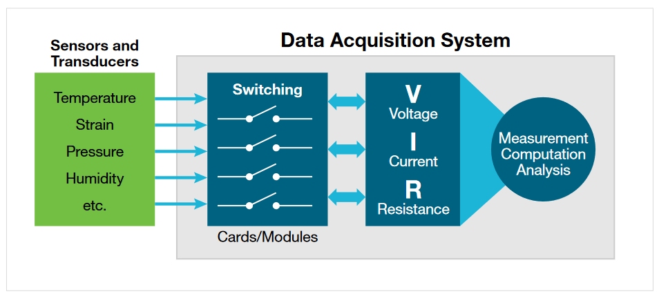
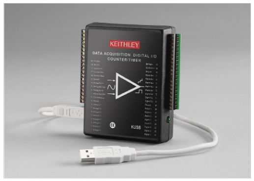
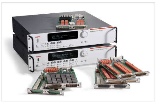
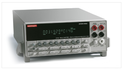
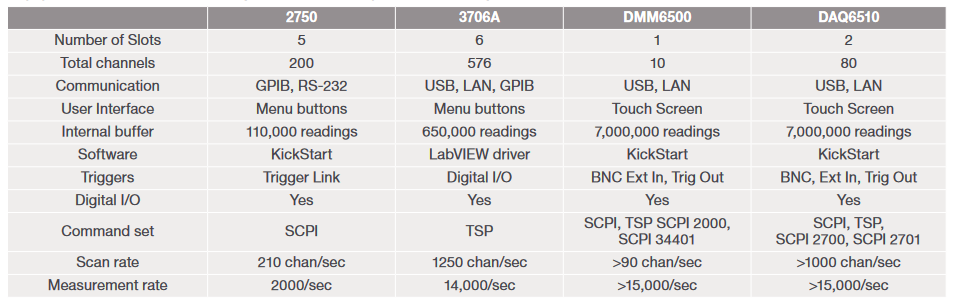
Data acquisition systems can be large or small, depending on the number of devices or sensors to be tested with one instrumentation setup. System costs will vary widely, depending on system requirements such as measurement accuracy, sensitivity, resolution, test speed, and the range of signal types that will be encountered. The USB unit shown here is an example of a low-cost option with marginal accuracy that can monitor a few items with one test setup. In contrast, the Keithley 3706A System Switch/Multimeter is a more sophisticated system that can test up to 576 devices with one test setup and measure with 7½-digit resolution and high accuracy.
The reason for choosing one over the other (or something in between) is completely user- and situation-dependent, but it all eventually comes down to weighing the price/performance tradeoffs involved:
- What is needed in the way of channel count, measurement accuracy, measurement speed, and possible additional features?
- Traceability – What degree of calibration is necessary for the equipment? Does the equipment need to adhere to certain quality standards as recommended or required by the automotive, aerospace, medical, or other industry?
- What does the equipment manufacturer provide in the way of support? Does their documentation promote ease of use and get the customer up and running quickly? Do they provide software or drivers and how practical are they?
Typically, an application that demands higher channel counts, speed, traceability, calibration, etc. will demand a more expensive data acquisition system. Although higher cost might initially seem like a bad thing, selecting the wrong tool for the job and regretting it later is far worse.
Who Uses Data Acquisition and Why?
Data acquisition hardware and software are widely used by engineers and research scientists in a broad range of industries and applications to gather the information they need to do their jobs better. The following list includes just a few of the numerous possibilities that data acquisition allows.
Condition Monitoring Applications
- Continuous monitoring of plant equipment or other assets for extended periods.
- Spotting problems early before a system failure occurs.
- Alerting maintenance personnel when an error occurs.
PC-Based Control and Automation Applications
- Controlling processes without operator intervention.
- Regulating equipment operation.
- Automating processes using open-loop and closedloop control.
Research and Analysis Applications
- Characterizing and recording behaviors or properties
- Studying natural phenomena
- Researching new products and designs
Design Validation and Verification Applications
- Confirming that a product or system meets its design specifications
- Establishing evidence that a product meets its users’ needs
- Testing adherence to an industry standard
- Testing over an environmental parameter range (temperature, humidity, pressure, altitude)
- Reliability testing (HALT, HASS, AST)
Manufacturing and Quality Test Applications
- Performing functional and system-level product test
- Product soak or burn-in
- Executing end-of-line pass/fail quality testing
- Inspecting for non-compliant products and subsystems
Relay Types and Switch Card Options for Making Multi-Channel Measurements
When discussing data acquisition, it is often directly tied to the idea of using relays to switch signals. Switching helps to increase channel count economically where signal conditioning and analog-to-digital conversion hardware can be shared among channels sequentially
Designing the switching for a data acquisition system demands an understanding of the signals to be switched and the tests to be performed. Requirements can change frequently, so automated systems should provide the flexibility needed to handle a variety of signals. Even simple systems often have diverse and conflicting switching requirements. The test definition will determine the system configuration and switching needs. Given the versatility that data acquisition systems must offer, designing the switching function may be one of the most complex and challenging parts of the overall system design. A basic understanding of relay types and switching configurations is helpful when choosing an appropriate switch system.
Relay Types
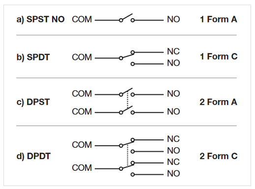
Understanding how relays are configured is critical to designing a switching system. Three terms are commonly used to describe the configuration of a relay: pole, throw, and form. Pole refers to the number of common terminals within a given switch. Throw refers to the number of positions in which the switch may be placed to create a signal path or connection. Contact form, or simply form, is a term used to describe a relay’s contact configuration. “Form A” refers to a single-pole, normally-open switch. "Form B" indicates a single-throw, normally-closed switch, and "Form C" indicates a single-pole, double-throw switch.
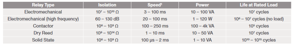
Common relay types include electromechanical, dry reed, and solid state. Some key parameters of each relay type are outlined in Table 1.
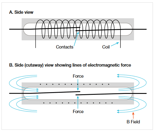
Electromechanical Relays
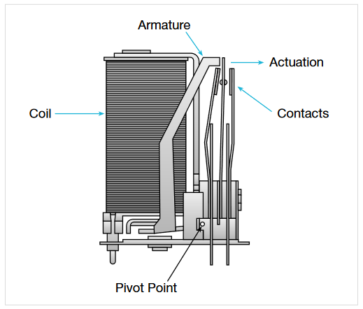
Electromechanical relays have a coil of wire with a rod passing through the middle (forming an electromagnet), an armature mechanism, and one or more sets of contacts. When the coil is energized, the electromagnet attracts one end of the armature mechanism, which in turn moves the contacts. The following figure shows a typical electromechanical relay with the main operating elements labeled and a scheme for actuating the armature. The coil must generate a strong field to actuate the relay completely
Electromechanical relays are available in configurations ranging from 1 Form A or B to 12 or more Form C. This type of relay can be operated by AC or DC signals and can switch currents up to 15 amperes, as well as relatively low-level voltage and current signals.
Electromechanical relays are available in non-latching and latching types. Non-latching relays return to a known state when power is removed or lost. Latching relays remain in their last position when relay drive current is removed or lost. Return mechanisms (for non-latching relays) and latching mechanisms can be magnetic or mechanical, such as a spring.
Because latching relays do not require current flow to maintain position, they are used in applications with limited power. In addition, the lack of coil heating, which minimizes contact potential, makes latching relays useful in very low voltage applications.
High Frequency Electromechanical Relays
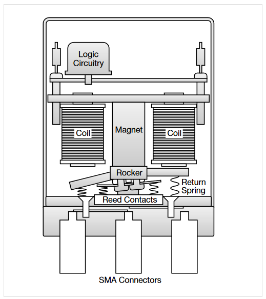
The capacitance between poles degrades AC signal isolation by coupling the signal from pole to pole or relay to relay. These capacitances within relays are a common factor that limit the frequency of switched signals. Specialized contacts and architecture are used in electromechanical relays to obtain good performance for RF and microwave switching up to 40GHz. A typical configuration is shown here, where the common terminal is between two switched terminals. All signal connections are coaxial to ensure signal integrity. In this case, the connectors are the female SMA type. For more complex switching configurations, the common terminal is surrounded by switched terminals in a radial pattern.
Dry Reed Relays
Dry reed relays are also operated by energizing a coil, but in this type of relay, the coil is wound around the switch so that the induced magnetic field closes the switch. Figure 7 shows a simplified representation of a typical reed relay. The switch is made from two thin, flat strips of ferromagnetic material called reeds with contacts on the overlapping ends. Leads are connected to the outside ends of the reeds and the entire assembly is sealed in a hermetic glass tube. The tube holds the leads in place (with a small gap between the contacts for normally open switches). Normally closed switches, less common than normally open, are made in one of two ways. The first method is to make the switch so that the contacts are touching each other. The second method uses a small permanent magnet to hold normally open contacts together. The field from the coil opposes the field of the magnet, allowing the contacts to open.
Solid State Relays
Solid state relays are typically comprised of an opto isolator input, which activates a solid state switching device such as a triac, SCR, or FET, with the latter one foremost for measurement and the former ones for control purposes. Reliability and longevity are some key differentiators. Although these are the fastest switching elements when actuation times are compared, the release, or turnoff time, is somewhat longer. AC control is a normal application for triacs and SCRs because the turnoff time is decreased when the device is switched off during a zero crossing. In addition, their isolation is limited by the leakage currents of the semiconductor devices, and they have a high insertion loss for low-level signals.
Switch Card Configuration Options
As a signal travels from its source to its destination, it may encounter various forms of interference or sources of error. Each time the signal passes through a connecting cable or switch point, the signal may be degraded. Careful selection of the switching hardware will maintain the signal integrity and the system accuracy
Scanner Switching
The scan configuration or scanner is the simplest arrangement of relays in a switch system. As shown in the following figure, it can be thought of as a multiple position selector switch.
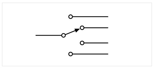
The scanner is used to connect multiple inputs to a single output in sequential order. Only one relay is closed at any time. In its most basic form, relay closure proceeds from the first channel to the last. Some scanner systems have the capability to skip channels.
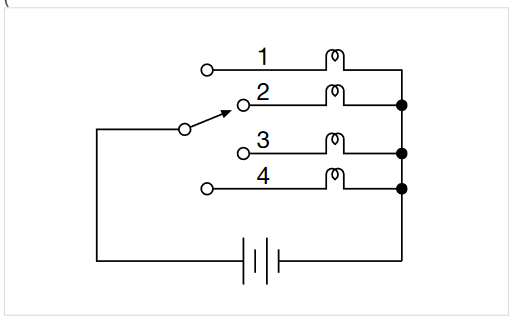
Figure 9 illustrates an example of a scan configuration. In this diagram, the battery is connected to only one lamp at a time, such as in an elevator’s floor indicator system. Another example is a scanner for monitoring temperatures at several locations using one thermometer and multiple sensors. Typical uses of scanner switching include burn-in testing of components, monitoring time and temperature drift in circuits, and acquiring data on system variables such as temperature, pressure, and flow.
Multiplex Switching
Like the scan configuration, multiplex switching can be used to connect one instrument to multiple devices (1:N) or multiple instruments to a single device (N:1). However, the multiplex configuration is much more flexible than the scanner. Unlike the scan configuration, multiplex switching permits multiple simultaneous connections and sequential or non-sequential switch closures.
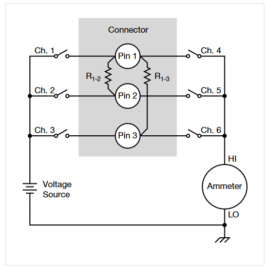
One example of a multiple closure would be to route a single device output to two instruments, such as a voltmeter and a frequency counter. The figure below illustrates another example of multiplex switching. This diagram shows measuring the insulation resistance between any one pin and all other pins on a multi-pin connector. To measure the insulation resistance between pin 1 and all other pins (2 and 3), close channels 2, 3, and 4. This will connect the ammeter to pin 1 and the voltage source to pins 2 and 3. The insulation resistance is the combination of R1-2 and R1-3 in parallel as shown. Note that in this application, more than one channel is closed simultaneously in non-sequential order.
Matrix Switching
The matrix switch configuration is the most versatile because it can connect multiple inputs to multiple outputs. A matrix is useful when connections must be made between several signal sources and a multi-pin device, such as an integrated circuit or resistor network. Using a matrix switch card allows connecting any input to any output by closing the switch at the intersection (cross point) of a given row and column. The most common terminology to describe the matrix size is M rows by N columns (M×N). For example, a 4×10 matrix switch card has four rows and ten columns. Matrix switch cards generally have two or three poles per cross point.
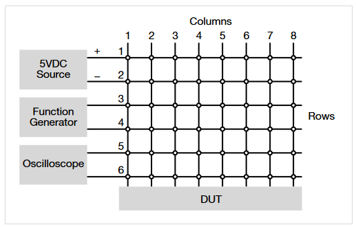
As shown in Figure 11, a 5VDC source can be connected to any two terminals of the device under test (DUT). A function generator supplies pulses between another two terminals. Operation of the DUT can be verified by connecting an oscilloscope between yet another two terminals. The DUT pin connections can easily be programmed, so this system will serve to test a variety of parts.
When choosing a matrix card for use with mixed signals, some compromises may be required. For example, if both high frequency and low current signals must be switched, take extra care when reviewing the specifications of the card. The card chosen must have wide bandwidth as well as good isolation and low offset current. A single matrix card may not satisfy both requirements completely, so the user must decide which switched signal is more critical. In a system with multiple cards, card types should not be mixed if their outputs are connected together. For example, a generalpurpose matrix card with its output connected in parallel with a low current matrix card will degrade the performance of the low current card.
Isolated Switching
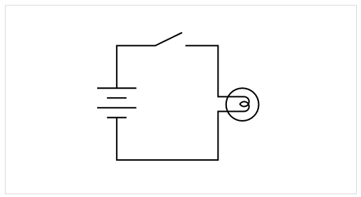
The isolated or independent switch configuration consists of individual relays, often with multiple poles, with no connections between relays. Figure 12 illustrates a single isolated relay or actuator. In this diagram, a single-pole normally open relay is controlling the connection of the voltage source to the lamp. This relay connects one input to one output. An isolated relay can have more than one pole and can have normally closed contacts as well as normally open contacts.
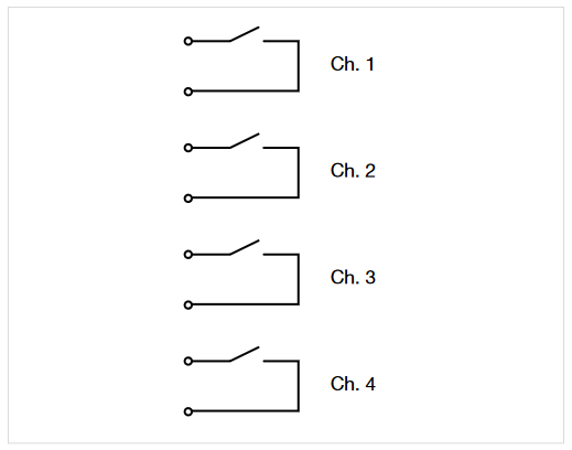
Given that the relays are isolated from each other, the terminals of each channel on the switch card are independent from the terminals of the other channels. As shown in Figure 13, each isolated Form A relay has two terminals. Two-pole isolated relays would have four terminals (two inputs and two outputs). A single Form C isolated relay would have three terminals.
Isolated relays are not connected to any other circuit, so the addition of some external wiring makes them suitable for building very flexible and unique combinations of input/output configurations. Isolated relays are commonly used in power and control applications to open and close different parts of a circuit that are at substantially different voltage levels. Applications for isolated relays include controlling power supplies, turning on motors and annunciator lamps, and actuating pneumatic or hydraulic valves.
Common Data Acquisition Measurement Types
Data acquisition systems can be configured to acquire information on a wide range of physical phenomena, such as pressure, flow, speed, acceleration, strain, frequency, humidity, light, and hundreds more. However, the four most commonly used measurement types are temperature, voltage, resistance, and current.
Temperature
Measuring temperature accurately is critical to the success of a broad array of applications, whether they are performed in industrial environments, process industries, or laboratory settings. Temperature measurements are often required in medical applications, lab-based materials research, electrical/electronic component studies, biology research, geological studies, electrical product device characterization, and many other areas.
Engineers from a number of disciplines (thermal, electrical, and mechanical) are concerned with how their products and devices perform in various environmental conditions. Having the appropriate measurement equipment helps them capture behaviors that cannot be witnessed by simple observation.
Typical temperature measurement applications
Thermal profiling: Measuring a device’s temperature over its range of use is important to understanding the stresses created at various temperature points and their effect on the life of the device under test. In addition, identifying hot and cold spots of the device during typical use can help designers minimize thermal effects.
HALT/HASS: Highly Accelerated Life Testing and Highly Accelerated Stress Screening are proven accelerated product reliability testing methods focused on finding defects in products so they can be fixed before they result in expensive field failures. They subject a product to a series of overstresses, including thermal ones, effectively forcing product weak links to emerge by accelerating fatigue. Stresses are applied in a controlled, incremental fashion while the unit under test is continuously monitored.
Product development: Accurate temperature measurements are critical during product development to allow engineers to understand how the product responds in various thermal situations.
Common temperature transducer types
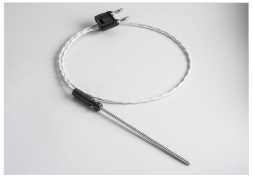
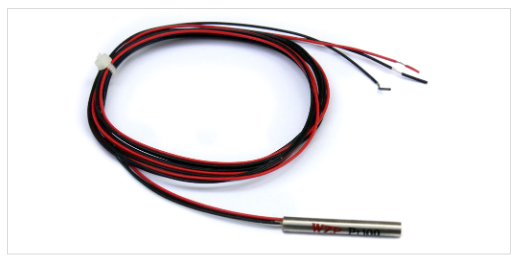
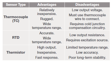
Thermocouples: Thermocouples (TCs) are formed by the junction of two dissimilar metals. Several different types, covering a wide temperature range, are available. Thermocouple linearity varies, depending on thermocouple type and temperature range. Of all the different types of sensors available to measure temperature, the thermocouple is by far the most common, mainly because thermocouples are relatively inexpensive, extremely rugged, and can be located long distances from the data acquisition system itself. However, connecting thermocouples can sometimes pose a challenge. In the case of higher-end data acquisition systems, manufacturers will often provide direct termination of the wires to a card or module populated with terminal blocks. An advanced interface such as this may well include circuitry to promote automated cold junction correction, helping to eliminate complicated setups that include extra lengths of wire, an external reference (such as an ice bath), and the need to include an additional measurement point to monitor the external reference. However, if the user purchased a standard digital multimeter with only front or rear input selection, they are faced with getting the best connection possible being routed into terminals that were not designed for direct thermocouple mounting. One solution is to use a thermal bead thermocouple probe, where the terminations are made using a standard banana plug interface. Some models of multimeter do provide a specialized input for thermocouples with the standard thermocouple connector, but, more often than not, even these probes can be used with an adapter to get to the more common banana jacks.
RTDs: Resistance temperature detectors are made with metal wires or films (most common being platinum) with a resistance that changes with temperature. RTDs require an external stimulus to function properly, usually a current source. However, this current has a tendency to generate heat in the resistive element, which adds error in the temperature measurement. There are three different methods that can be used when making RTD measurements, each contributing to a higher degree of accuracy when applied, respectively: two-wire, three-wire, and four-wire. RTDs are significantly more accurate than thermocouples; however, they are somewhat more costly and not as rugged.
Thermistors: Thermistors, like RTDs, change resistance as temperature changes. They offer higher accuracy like RTDs and are easy to set up. Although thermistors are less linear than RTDs, the measuring instrument (such as a digital multimeter) will have built-in algorithms to help resolve this and maintain the elevated accuracy. While they have a limited range, thermistors have a quicker response to temperature changes than the alternatives. A thermistor’s resistance changes more for a given change in temperature than does the resistance of an RTD.
Temperature Sensor Comparison
Temperature measurement best practices
- Take the time to weigh which sensor will be the most appropriate for the specific application.
- Consider the required measurement accuracy and speed.
- Determine how many points of measurement are required. Some temperature data loggers can scan and monitor many channels.
Strain
Studying the physical behavior of mechanical structures frequently includes measuring strain, which is defined as a physical distortion of an object in response to one or more external stimuli applied to the object. Typical stimuli include linear forces, pressures, torsion, and expansion or contraction due to temperature differentials. Strain can result in elongation or contraction; these phenomena are noted by the use of a (+) sign for expansion or a (–) sign for compression.
Strain information is important in structural engineering because it can be used to determine the stress present in an object. Stress data can then be used to assess factors such as the structural reliability and service life of the object. The basic principle of strain measurement is also used in other types of force-related measurements, such as pressure, torque, and weight.
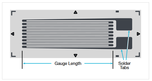
Strain is calculated as the change in length of an object divided by the unit length of the object. Normally, this change is extremely small in relation to the object’s length. Strain gauges or sensors are designed to provide a measurable signal (voltage, resistance, or current) to determine the degree of distortion caused by the items in question.
Typical strain measurement applications
Load Cells, Pressure Sensors, and Flow Sensors: A variety of physical phenomena can be measured with strain gaugebased transducers coupled with specialized mechanical elements. These phenomena include load, gas or liquid pressure, and flow rate, among others.
A load cell is simply a packaged strain gauge designed to measure force under different load conditions. A typical load cell body is machined from metal to provide a rigid but compressible structure. The load cell body is usually designed with mounting holes or other fittings to allow the unit to be mounted permanently on a supporting structure.
Typical transducers for pressure sensing are electromechanical devices that combine a sensor with mechanical elements such as a diaphragm, piston, or bellows. The mechanism is designed to respond to a pressure differential and expand against a spring, which determines the range of the sensor. The pressure-sensing element also actuates a strain or positional sensor that produces an electrical output that can be read by an instrument.
Flow can be measured in a variety of ways, most of which are indirect measurements that depend on the material’s viscosity, conductance, or other properties. One very common way to infer flow is to use two pressure sensors to measure the material’s pressure drop when passing through an orifice.
Acceleration, Shock, and Vibration: Acceleration, shock, and vibration are important parameters in mechanical applications, including automotive, aerospace, product packaging, seismology, navigation and guidance systems, motion detection, and machine maintenance. These parameters can all be measured using a sensor known as an accelerometer.
Acceleration is the rate of change of velocity that a mass undergoes when it is subjected to a force. It is defined by the formula: force = mass × acceleration.
Assuming that mass and force remain the same, then acceleration is constant, meaning that an object’s velocity will continue to change at a uniform rate. Acceleration is expressed as distance per time squared, with meters/sec2 and feet/sec2 being common units. Earth’s gravity exerts a force of 9.8m/sec2, or 32ft/sec2; this amount of acceleration is often referred to as 1g (g for gravity). Sensors designed to measure acceleration can measure values ranging from millionths of a g (μg) to hundreds of g or more. They are frequently designed to withstand overloads of thousands of g without damage.
Shock is a special case of linear acceleration in which the acceleration (or deceleration) time approaches zero. In the real world, the time cannot equal zero, but it can equal a very small fraction of a second. The result of a large change in velocity over a short time can produce an acceleration of hundreds of g or more.
For shock studies, the measurement range of the accelerometer must be able to handle the acceleration expected in the specific shock situation. This value can be calculated by dividing the change in velocity by the time interval:
Vibration is a continuing change in the position of a body, typically occurring in a cyclic pattern with a constant or near-constant period. Vibration is a common characteristic of machines; it is of interest in manufacturing because its measurement can provide an indication of the health of machinery. Periodic monitoring and analysis of vibration levels can reveal specific problems, such as worn bearings, loose fasteners, or out-of-balance rotating components, before they become severe enough to be noticed or to cause complete failure. Vibration is a cyclic changing of position, so it can be detected by using an accelerometer.
Voltage
Like temperature, voltage is very commonly measured with data acquisition systems. Most electrical measurement devices (voltmeters, digital multimeters, etc.) measure voltage but offer different measurement ranges, sensitivity, accuracy, and speed.
Typical voltage measurement applications
Monitoring the voltage output of a transducer. A transducer converts a mechanical parameter into an electrical parameter, typically a voltage. In addition to the temperature transducers described previously, examples of transducers include strain gauges, pressure gauges, humidity sensors, and ultrasonic sensors.
Monitoring the voltage output of an electronic device or an internal circuit of an electronic device. Voltage measurements verify that a product or device meets its specifications or performs as required. The product or device is tested under varying conditions to ensure the product meets its specifications, and numerous voltage measurements are often required. Internal circuit voltages are monitored to ensure that circuits perform properly under a wide range of test conditions.
DC Voltage vs. AC Voltage
Direct current (DC) refers to a unidirectional flow of electric charge. DC voltages can be produced by sources such as batteries, power supplies, thermocouples, solar cells, or dynamos. DC voltages may flow in conductors such as wires, but they can also flow through semiconductors, insulators, or even through a vacuum, as in electron or ion beams. In alternating current (AC) circuits, rather than a constant voltage supplied by a battery, the voltage typically oscillates in a sine wave pattern that varies with time. In household circuits, the AC voltage oscillates at a frequency of 60 Hz. Frequency and period measurements are part of the AC measurement family. Frequency is a measurement of the number of cycles per second; period is a measurement of the time period of the AC wave.
Common voltage measurement challenges
Input impedance of the voltmeter: The voltmeter has a limited amount of impedance. When connected to the source of the voltage to be measured, if the source impedance is of sufficient magnitude, the input impedance could cause an error in the measurement. Most voltmeters today offer a choice of two input impedances, 10 MΩ and 10 GΩ. Typically, the higher the input impedance used, the less the voltmeter will affect the source voltage.
Resolution of the voltmeter: Voltmeters can offer anywhere from 3½ digits to 8½ digits of resolution. For quick and crude voltage measurements, choose a low-resolution voltmeter. For more accurate and stable voltage measurements, use higher-resolution instruments.
Resistance
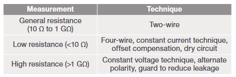
Resistance is another commonly measured parameter in data acquisition systems; it can be measured by either of two methods: constant voltage or constant current. The constant voltage method sources a known voltage across an unknown resistance and measures the resulting current, then calculates the resistance. This method is widely used for high resistance measurements (>1 GΩ).The constant current method sources a known constant current through the unknown resistance and measures the resulting voltage. Then the resistance is calculated. This is normally used for resistances <1 GΩ.
Typical resistance measurement applications
Measurement of resistive devices is performed to ensure the magnitude of the resistance is within specification. Many resistive devices have temperature coefficients, which means the resistance varies with temperature. These characteristics need to be verified over a temperature range.
Measurement of contact resistance. Contact resistance is the resistance to current flow through a closed pair of contacts. These types of measurements are made on components such as connectors, relays, and switches. This resistance is normally very small, ranging from micro-ohms to a few ohms.
Measurement of isolation resistance on multi-pin connectors and multiple wire cables. This is done to ensure that there are no unintended connections or shorts between independent connector pins and wires.
Measuring the resistance or resistivity of a material such as a polymer. The resistance can be used to gauge the material’s ability to hold or dissipate charge that may accumulate, such as on a static-sensitive mat.
Two-wire vs. four-wire resistance measurements
The two-wire resistance measurement technique uses the same two leads for sourcing and sensing. This means that a current is forced through the wires and the voltage is sensed with the same wires. Note that the voltage is sensed at the meter terminals and not at the resistive device. This technique is convenient and simple to use; for most resistance measurements, simply connect the two wires to the circuit of interest and make the measurement.
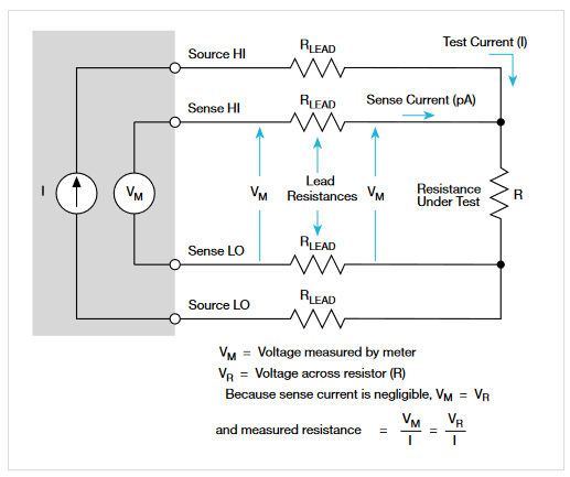
The four-wire technique sources a current with two wires and senses the voltage drop using a different set of two wires. This allows the voltage to be detected at the resistance under test. The four-wire technique has the advantage of eliminating test lead resistance because it measures the resistive device and not the test lead resistance. Test lead resistance is generally several hundred milli-ohms in magnitude and represents a large offset in a low resistance measurement.
Common resistance measurement challenges
Low resistance measurement with a two-wire measurement device: To eliminate test lead resistance, most ohmmeters and digital multimeters include a feature called ZERO, NULL or Relative. Using this feature is a two-step procedure. First, the two test leads are shorted together. Second, enable the ZERO, NULL or Relative feature, which will subtract the measured short-circuit resistance from every subsequent reading.
When high resistance measurements are too low: When making high resistance measurements (1 GΩ and higher), the instrument setup itself can introduce problems. Follow these steps to prevent these problems:
- Low insulation resistance: The test fixture’s insulation resistance could be in parallel with the device under test.To remedy this problem, use a test fixture and connecting cables with higher insulation resistance. A driven guard can also effectively increase shunt resistance.
- Input resistance of the voltmeter is too low for the measurement: Use the force voltage and measure current technique
Offset current: Offset current may be caused by charge stored in the material being measured. Adjust the meter’s zero baseline to compensate for offset current or use the alternating polarity method to cancel these offsets.
Low resistance thermoelectric errors: Measuring low resistance is really a matter of measuring low voltage; thermoelectric EMFs in the circuit are major sources of error in low voltage measurements. To correct this, use offset compensation. The first step in the technique is to force the current in the positive polarity and take a voltage measurement. Then, force a current of the same magnitude to the negative polarity and take another voltage measurement. Then add up the voltages and divide by two.
This yields a "compensated" resistance measurement that eliminates the thermoelectric effects.
The following table summarizes resistance measurement techniques and the supplemental corrective functions that can be applied to enhance each.
Current
Current measurements are used to determine resistance, power and, of course, current flow in a circuit. Unlike voltage measurements, current measurements cannot be made by simply placing the test leads across the sample. Instead, in a standard shunt-style current measurement, the current path is broken and a current shunt placed in series so that when the current flows through the shunt, it develops a voltage. With the shunt resistance value known and the voltage measured, the current can be calculated.
Typical current measurement applications
- Monitoring the power consumption of a device under test (DUT) by measuring the current drawn from the DUT
- Measuring the current from transducers that have 4–20 mA outputs
- Determining the maximum current output of a device under various operating conditions
DC current measurement techniques
The traditional (shunt-style) current method requires breaking the circuit and placing a shunt resistance in series with the break. When the current flows through the shunt resistance, a voltage is developed that is measured. Dividing this voltage measurement by the known shunt resistance yields the current. This is the standard method employed in most current measuring circuits in instruments like digital multimeters (DMMs). The smaller the anticipated current is, the larger the shunt resistance should be. So, for measuring microamps of current, usually a 100 kΩ or 1 MΩ shunt is used. At higher current levels, the shunt resistance is lower; for ampere-level measurements, usually a 1 Ω or even a 0.001 Ω shunt is used. It all depends on the level of current anticipated and the voltage drop across the shunt.
The active shunt or feedback ammeter method also requires breaking the circuit and placing the ammeter in series with the break but inserting an input to an active operational amplifier (op amp) rather than a shunt resistance. The feedback of the op amp determines the level of current that can be measured. This method is usually appropriate for low current measurements, so it is employed in picoammeters and electrometers.
AC current measurement technique
AC current measurements are DC current measurements in which the AC signal is routed through an AC–to-DC converter. The shunt-style method is generally used in AC current measurements: the current flows through the shunt, the voltage drop is measured and then routed through the AC-to-DC converter. The bandwidth is important for AC current measurements. With most AC current meters, the bandwidth is up to about 5 kHz.
Common Current Measurement Challenges
Voltage burden is an error term in current measurements resulting from having to insert the measurement instrument into the circuit under test and having to build up a voltage in the circuit to compute current. With shunt-style current measurements, the voltage dropped across the shunt can be significant, which can reduce the current to be measured. With a feedback ammeter, the voltage burden is the offset of the differential input of an operational amplifier, which is usually very low (millivolts to microvolts). The lower the voltage burden due to the measurement technique, the more accurate the current measurement.
Guidelines for Selecting a Data Acquisition System
To configure a data acquisition system appropriately, it is vital to define application requirements early. Answering these questions will provide valuable guidance during the equipment selection process:
- What kinds of signals are to be measured? This could be voltage, current, resistance, etc.
- What is the magnitude of the signals to be measured? This could range from microvolts to kilovolts or picoamps to amps, or milliohms to gigaohms.
- How many signals are to be routed and measured? This answer can help determine how many measurement channels are required and allows narrowing down equipment options.
- What test timing issues are important? What acquisition rate is needed? How long will the tests last—minutes, hours, days, weeks? Some production tests can be completed in seconds, but the equipment operates 24/7. For this type of around-the-clock data acquisition, switch relay life must be taken into consideration. Although most relays can withstand millions of open/close cycles, the level of signals being routed can affect lifespan.
- What level of accuracy is required for each parameter in the test? There is typically some level of tradeoff between accuracy and acquisition rate. Generally, the higher the rate, the less accurate the measurements will be.
- How much data must be collected? Many data acquisition systems have internal buffers. Generally, saving data to these buffers offers the fastest method of obtaining data and is a good approach if the amount of data to be acquired is less than the instrument’s storage capacity. However, if the data must be displayed in real time on a screen, a different approach will be acquired. If the system includes a PC with a USB port, lots of data can be saved to a USB drive.
- How big is the equipment budget? Cost will always be a major factor in selecting a data acquisition system. The cost per channel is one factor in the cost of the system. What types of switching relays are required (electromechanical, reed, or solid state)? Because relays are mechanical in nature, they have limited lifespans. How often will that lifespan be reached? Factor the relay life into the cost equation.
Software Support for Data Acquisition Equipment
Knowing that the data acquisition equipment selected for a task is capable of performing it properly is critical, but learning how to use it can often be the greatest challenge. Many users rely on a software interface to become familiar with the basic functionality of their instrumentation and gradually work their way up to more complex scenarios. The software tools chosen need to balance intuitive operation and high ease of use with sophisticated test development capabilities to simplify the transition from ensuring proper functionality at the benchtop to developing a series of commands that optimize the instrument’s performance in a production environment. Keithley products are compatible with an array of software options, which are outlined in the following sections.
At the Bench and in the Lab
The expression "bench software experience" refers to a user’s hands-on interaction with a test instrument that is not connected to an external computer. The firmware embedded in the instrument is the first “software” the user encounters because it is immediately available through the front panel of the instrument on the benchtop. A traditional front panel interface provides an array of buttons and soft keys (also typically tied to actual buttons) that allow modifying the settings and properties of the measurement behavior that is active on the instrument. A multi-line alphanumeric liquid crystal display (LCD) shows the actual menu options and measurements to reflect the current state of the instrument.
The test and measurement industry has employed traditional interfaces like these for decades, and several Keithley data acquisition instruments that incorporate them are still available. When this interface is used with a quick-start or user’s guide (either printed or electronic), users can gain familiarity with their instrument simply by following the steps listed in the guide.
A new user experience and why it is important
The growing use of smartphones and tablet PCs have led consumers to expect more from their electronic devices than a nice-looking display. These devices not only enhance the viewing of desired content but also allow the user to assume a more interactive role in how the software applications respond to them. This makes the experience more intimate and builds a personal foundation between man and machine. Much the same is true with test instrumentation. College and university students are using touchscreen test equipment as part of their coursework. Soon those students will be the next wave of new engineers, building technologies that will shape the world in previously unimaginable ways. Modern instrument interfaces will not just be demanded, they will be expected.
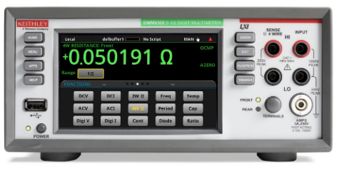
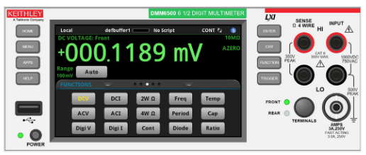
Keithley’s most recent products are equipped with touchscreen interfaces in an effort to clean up the front panel, speed instrument setup, simplify access to settings and features, and allow users to begin analyzing results faster. These instruments bring actions commonly used with tablets or smartphones (swipe, poke, pinch and zoom) to the benchtop, providing a more logical flow for how "everyday measurement" should take place. The touchscreen interfaces simplify getting test results quickly and with the high accuracy. These touchscreen instruments offer:
- An intuitive interface that minimizes the user’s learning curve
- Easy navigation between set-up and configuration menus for fewer errors
- Real-time graphing, data visualization, and onscreen analysis
Engineers often say, "I will use this primarily in a rack or system with a remote interface, so the front panel is not a big deal to me." However, that point of view often changes when a problem arises that forces the engineer to troubleshoot by methodically manipulating the equipment configuration to find the source of error. Having the power to debug an issue more effectively and share this capability with support technicians on the production floor can save considerable time.
The touchscreen user experience (UX) offers an alternative to the remote software interface, removing the PC and the cabling to connect it to the instrument from the work area.
The set-up screens simplify test configuration in much the same way as a secondary desktop software would and offer graphing, cursors, and statistical information on the acquired measurements to allow for immediate analysis of results.
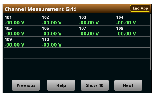
Additionally, a flexible, smart software interface can simplify bringing customized applications and setups directly to the test equipment without the need for a firmware upgrade or external software. This might include regular benchtop setups or custom-built diagnostics tools. For example, some users might want their data acquisition system to make the measurements across multiple channels more viewable or need some maintenance tools for monitoring the life of switch card relays to alert them when they are approaching "end-oflife" conditions prior to getting degraded performance.
Access equipment with the embedded web interface from a web browser
For those users who prefer working with a larger screen, some test instruments also include an embedded web server that can be used with a choice of web browsers, including Microsoft® Internet Explorer or Edge, Mozilla Firefox, Google Chrome, and Apple Safari. The web interface (Figure 22) simplifies reviewing instrument status, controlling the instrument, and upgrading the instrument over a LAN connection.
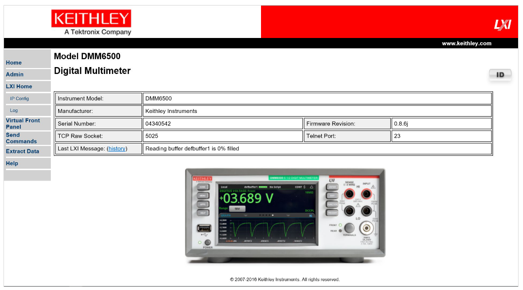
The instrument web page resides in the firmware of the instrument. Changes made through the web interface are immediately made in the instrument. Some of the web tools will allow typing in and issuing remote commands just as if they were sent via custom control software. For instance, on some data acquisition systems, examples from manuals can be run through an embedded web application that is available on the instrument’s web interface.
Some instruments’ embedded web interfaces feature a virtual front panel page that allows controlling the instrument from a computer in much the same way as using the front panel. The instrument can be operated by using a mouse to select options. This can be a valuable feature for users who want to configure and check in on their tests from another location.
Instrument Control Software
No matter how rich a user interface is built into a data acquisition system, it can still be advantageous to work with a piece of software that extends the control of the instrument to an external computer. The mindset here is to avoid getting bogged down in the minutiae of programming. The system creator knows the kind of equipment needed for the test but does not have the time to learn every little detail about it. He or she knows the application, the stimuli that must be applied, and the measurements to be made. What is needed is a software package that promotes minimal effort in instrument setup, and provides data analysis where results and images can be immediately added to the project’s documentation or formal report. Ideally, the software in question would have the application structure already built into it. Fortunately, several test instrumentation manufacturers have solutions for just this situation.
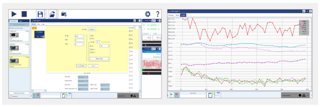
Keithley’s KickStart is PC-based software that manages both the instrument configuration and execution of tests. It provides a simple interface to the instrument so that users can gather test insights without becoming instrumentation experts. Users can be up and running with their instrument(s) in minutes as KickStart accelerates their learning curve by automating data collection from multiple instrument without programming. KickStart offers quick visualization of data and tools to compare data from test run history. Such features enable faster discovery of measurement trends and device dependencies on environmental conditions, for example. This aids the design engineer in making the necessary decisions to continue on to the next stage of the product development and aids the test engineer in validating the performance of the device or certifying that the device complies with a particular regulatory standard.
KickStart can capture millions of readings from the instrument and stream them directly to PC storage media for safe data archival. Users may save test configurations in order to replicate previous tests quickly and even create a library of tests for a particular device or compliance standard.
KickStart provides a variety of user conveniences for interacting with the data so that users can make faster decisions on what the data shows:
- Customize view of the data table to show and hide only the data of interest
- View plots of multiple measurements at once
- Assign meaningful labels to channels of the data acquisition switching card
- Get statistical overviews of data for each channel in the table
- Highlight/mark data points of interest on the graph
- Export data at any time during the test to share test updates with colleagues and stakeholders
In the System
When the experimental setups and equipment understanding are complete, it may be time to consolidate all test equipment. Individual elements are mounted into a rack, customized fixtures are created that route test paths to the DUT, and a common piece of test software that can sequence the tests to be executed in a production environment is generated. The bench and lab setups will have provided much of the hardware understanding needed, and the software control and optimization ends up becoming the critical final stage. Although there are a number of programming options from which to choose, the following are some of the most common for which Keithley provides solutions.
Leverage SCPI commands to control the system
Using Standard Commands for Programmable Instruments (SCPI) is most common for the majority of system integrators who also write their own control code. SCPI commands are provided in an easily readable ASCII format and help the user logically map a command to the function or attribute they wish to modify on the instrument in question. A series of commands can be over the communications interface of choice (USB, LAN, GPIB, or RS-232) to facilitate the handsfree automation that is desired for production.
Although SCPI is sometimes referred to as a programming "language," it should be noted that the language in question is one that is understood by test instrumentation, and should not be confused with conventional programming languages (C++, Visual Basic, and Python, for example). SCPI still requires the use of a separate programming tool to allow for sending commands and querying information.
IVI and LabVIEW instrument drivers
Instrument drivers provide a set of software sequences that control a remote, programmable instrument used for configuration, writing/reading, and triggering. These drivers help to cut test program development time by minimizing the user’s requirement for learning the programming conventions for each instrument. IVI (Interchangeable Virtual Instrument) drivers provide a generic wrapper around an instrument’s specific SCPI command set, allowing for instruments from different manufacturers to be used with the same driver. For example, test engineers accustomed to using DMMs produced by other companies could purchase a Keithley DMM and integrate it into their existing test systems without modifying their IVI-based control code.
Because of the highly generic nature of pure IVI drivers and the fact that instrument models provide custom features, instrument designers will often provide a more specific IVI driver that exposes the additional programming control available for the selected instrument model. Although this is in opposition to the promised interchangeability that strict IVI intends to provide, these additional features tend to offer the end user more than a one-size-fits-all model. Keithley provides IVI-C and IVI-COM drivers for its DMM and switching products that can be used with common programming development tools such as Microsoft Visual Studio, MATLAB®, Python and National Instruments’ LabWindows™/CVI. Installing the Keithley IVI drivers also provides examples in C, Visual Basic, and C# to offer users code that shows the actual application use cases for the instrument driver.
LabVIEW® is a software-based graphical programming environment that allows users to create programs showing the flow of both variables and data (through wires), and immediately have them presented on a user interface. LabVIEW is a visual tool intended for control and data presentation. It offers a building-block style that may be easier for those who do not consider themselves programmers to comprehend and become acclimated to than traditional text-based programming languages like C and Java. A program that would take several weeks to write using a text-based programming language could be completed in a fraction of that time using LabVIEW because it is designed for on-screen measurement configuration, data analysis, and results presentation. Because LabVIEW drivers use VISA as the underlying instrument communication tool to call underlying SCPI commands, the user also has the flexibility to choose equipment with a variety of protocols, including GPIB (General Purpose Instrument Bus), serial, USB, and Ethernet.
LabVIEW offers an extensive library function set to help users with most programming efforts. Keithley provides LabVIEW driver code libraries with application-specific examples for the target instrument, which can include multi-channel data acquisition, datalogging, single- and multi-point measurement, digitized measurements, and switching.
Although the use of IVI and LabVIEW drivers promises easyto-use and ready-made tools, using either of these choices still involves a learning curve. As noted, each leverages an instrument’s SCPI command set, and optimizing a test system almost requires users to become acquainted with the lower-level commands. Additionally, some studies indicate that direct use of an instrument’s SCPI command set provides a speed advantage over the IVI and LabVIEW options. Therefore, users need to weigh the advantages and disadvantages of each before beginning their programming efforts to ensure a balance of usability optimization for themselves and other team members involved in the development and maintenance of test system code.
Optimizing the system
For production test systems, it is important to investigate all options that can decrease test time and increase throughput. Presumably, at this point, the test equipment has been chosen using the considerations outlined in "Guidelines for Selecting a Data Acquisition System." With the hardware options covered and a clear understanding of the remote commands needed to control the instruments, the next task is constructing the software process that automates product testing. Although an obvious solution to increasing throughput might be to increase test system capacity, this may be neither immediately feasible nor necessary. The integrated programming environment (IDE) chosen probably provides options to multithread or multitask; also consider what the test instruments themselves offer with respect to promoting test speed.
It is also important to weigh how much built-in instrument intelligence the data acquisition system provides. Most test instruments allow saving a number of configurations to internal memory that can then later be recalled as needed. This can greatly reduce the number of overall command writes to the test instrument that the controlling PC would have to execute; this would allow storing a long series of commands on an instrument but only needing to send one command to have them all executed.
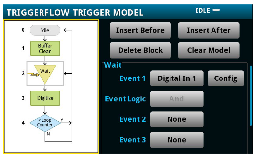
Now consider a series of instruments that must be set up or that must execute their desired actions all at the same time without the overhead of parallel processing on the PC side. One way to implement this parallel operation is through the triggering mechanisms that are available on the test instrumentation used. A variety of options are possible, either through dedicated trigger in and out ports, digital inputs/output lines, or other communication protocol triggers (such as LAN, GPIB, or PCI Express if these options are available). Test instruments will usually have a documented “trigger model” – a flow diagram that shows all the events and actions that are staged to perform the switching and/ or measurement. Studying such models can help users gain a deeper knowledge of the instrument-level processing and may lead to insights on how to optimize the testing scheme further. Even more advantageous is when the user is presented with the ability to circumvent using a dedicated trigger model and define their own to further remove any unnecessary processing that might otherwise slow the instrument.
A variety of other options should be considered when looking for ways to streamline testing:
- Use fixed ranging in lieu of auto ranging to remove any deciding logic that is applied in the instrument firmware. At this point, the anticipated test outcomes are already known so select a specific range and reap the benefits.
- Consider measurement quality vs. measurement speed tradeoffs. In a production setting where quantity may be valued over quality, it might be beneficial to reduce the integration time (or increase the sampling rate) to get results close to what the functional test is expecting. For example, reducing the aperture time from one power line cycle (1 PLC) to 0.01 PLC might not deliver the best 6½-digit resolution with an integrated measurement on a DMM, but it will deliver up to ten times faster readings.
- Leverage more mathematical and process control at the instrument level. If the test results require statistical information or data converted to values of a different unit of measure, use whatever built-in functionality the test equipment provides to help eliminate large data transfers and processor-taxing operations that might occur at the PC.
Many of these options will be standard features of the instrumentation, with others available as add-ons. Others might only be available through specific vendors, so take the time to seek out instrumentation that offers the capabilities most important to a particular application.
For example, Keithley instruments with Test Script Processor (TSP®) technology operate like conventional instruments by responding to a sequence of commands sent by the controller. Individual commands can be sent to a TSPenabled instrument the same way as any other instrument. TSP technology allows message-based programming, much like SCPI, with enhanced capabilities for controlling test sequencing/flow, decision-making, and instrument autonomy.
Unlike conventional instruments, TSP-enabled instruments can execute automated test sequences independently, without an external controller. A series of TSP commands can be loaded into the instrument using a remote computer or via the front-panel port with a USB flash drive. These commands can be stored as a script that can be run later by sending a single command message to the instrument, or loaded and run from the front panel. The primary tradeoffs are programming complexity vs. throughput. Relatively simple programming techniques will allow noticeable throughput improvements. Slightly more complex programming (using TSP-based instruments and programming best practices) can produce significantly higher throughput gains.
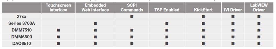
See Appendix B for examples of software options available for various Keithley data acquisition tools.
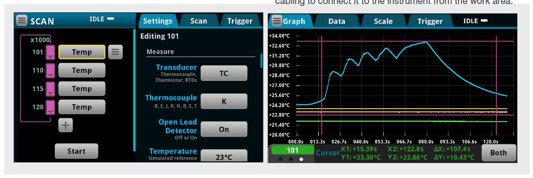
Example Application
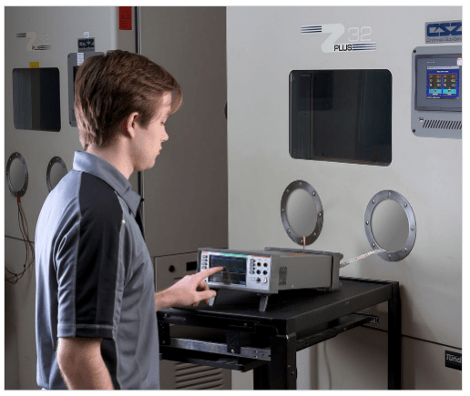
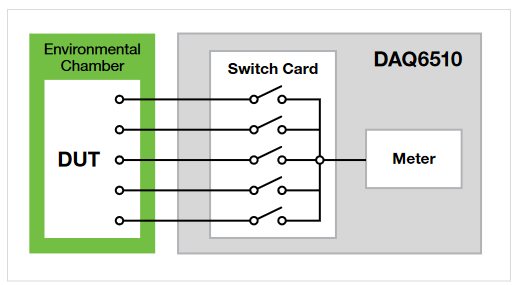
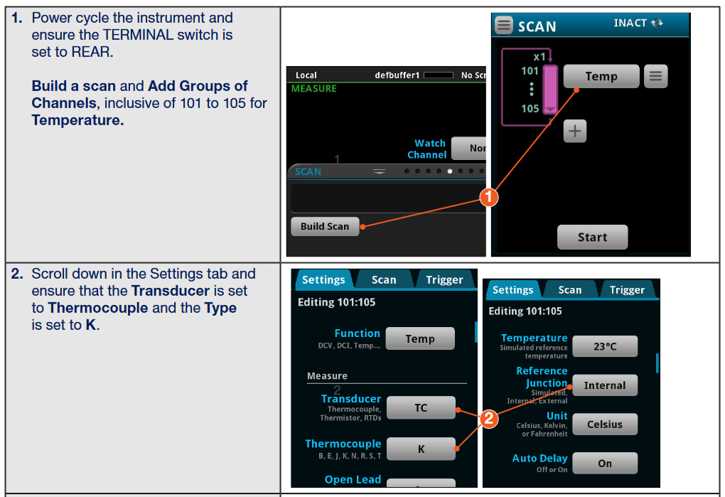
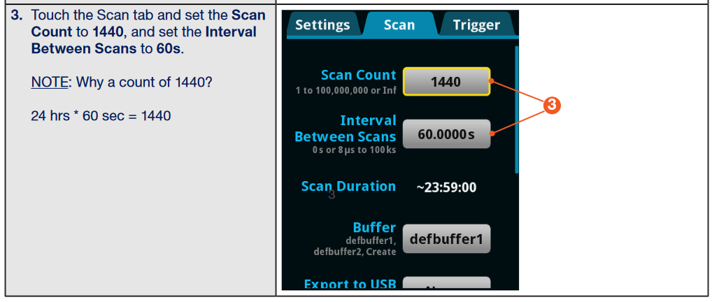
Performing a long-term temperature scan is a very common application for data acquisition instruments. This example employs a DAQ6510 with a 7700 Plug-In Switch Module for the data acquisition system, which will monitor the temperature on specific locations of a product in a temperature chamber.
- To keep the cost of the solution low while still covering a broad range of temperatures across five channels, the transducer of choice is the thermocouple.
- A Type K thermocouple type is used because it supports the widest range of temperatures; internal cold junction correction is employed to enhance the measurement accuracy by compensating for offsets that may present themselves at the connection of the thermocouple to the measurement channel.
- Thermal profiling of a device under test (DUT) can last for days, weeks, or up to a year. This example will run for 24 hours.
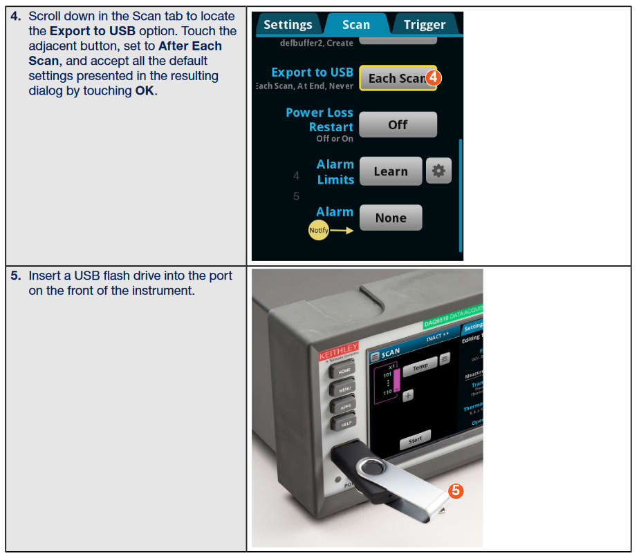
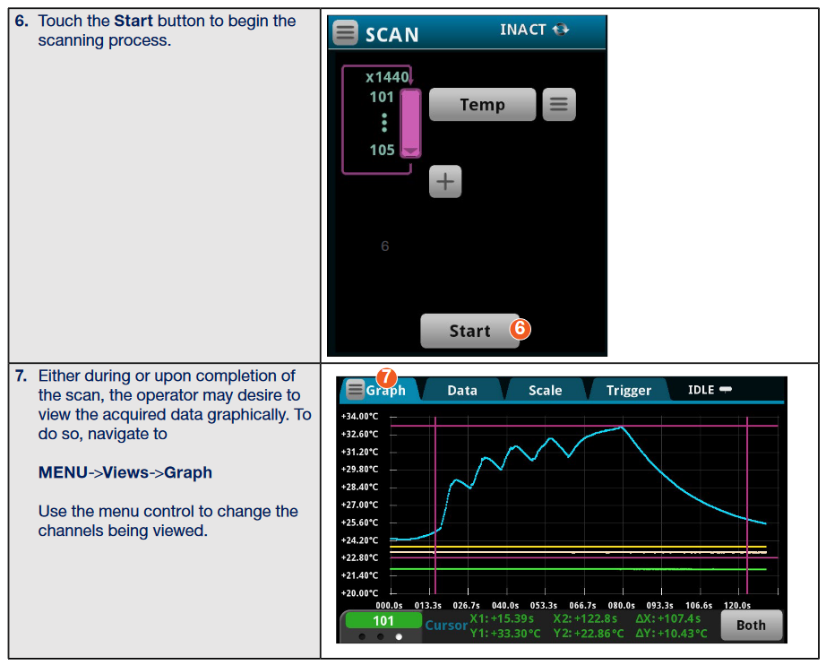
- Because lab setups can have limited resources, the setup will assume no PC is available, but the measured data must still be preserved. Therefore, the data will be exported to a USB flash drive for each of the scans executed.
Here is a general diagram of the test setup:
Conclusion
Understanding the intricacies of data acquisition can be quite a complex task. It is essential to determine the scale of the system required in terms of channel count and the accuracy of measurement hardware, as well as the switching type and topology that will be used to route the signals. The next step is understanding the types of measurements required for the application and seeking guidance on how and when to apply optimization techniques to those measurements. It is also important to consider all the software options for the equipment in question for applications that must make a transition from the lab to the production floor. Study everything that is available in the way of documentation—the application examples, demos, and videos, etc.—not just the standard manuals. Finally, consider the resources available to offer assistance with questions that the documentation cannot answer.
Appendix A: Keithley Data Acquisition Systems Overview
Appendix B: Software Support Tools Compatible with Keithley Instruments